Applying GI Detection Methods on Simulated Data
Delta Log Fold Change (dLFC) Application
Here, we show how we may apply dLFC [1] to calculate GI on simulated data, as an example to analyze the simulation output.
knitr::opts_knit$set(root.dir = getwd())
# read example simulated data
sample_name = "example_data"
pseudo_counts = 5e-07
repA_path <- here::here("data", paste0(sample_name, "_repA.csv"))
repB_path <- here::here("data", paste0(sample_name, "_repB.csv"))

# each simulation is containing two replicates A and B, and we take average of the LFC for analysis
cell_lib_guide2_A = read.csv(repA_path) %>%
  dplyr::select(-X)

cell_lib_guide2_B = read.csv(repB_path) %>%
  dplyr::select(-X) %>%
  dplyr::select(guide_id, counts_guide_t0,
                counts_guide_t1, counts_guide_t2,
                rel_freq_guide_t0, rel_freq_guide_t2, LFC)

cell_lib_guide2 = merge(cell_lib_guide2_A, cell_lib_guide2_B, by = "guide_id") %>%
  dplyr::rename(counts_guide_t0_1 = counts_guide_t0.x,
                counts_guide_t0_2 = counts_guide_t0.y,
                counts_guide_t1_1 = counts_guide_t1.x,
                counts_guide_t1_2 = counts_guide_t1.y,
                counts_guide_t2_1 = counts_guide_t2.x,
                counts_guide_t2_2 = counts_guide_t2.y,
                rel_freq_guide_t0_1 = rel_freq_guide_t0.x,
                rel_freq_guide_t0_2 = rel_freq_guide_t0.y,
                rel_freq_guide_t2_1 = rel_freq_guide_t2.x,
                rel_freq_guide_t2_2 = rel_freq_guide_t2.y,
                LFC_t2_1 = LFC.x,
                LFC_t2_2 = LFC.y) %>%
  mutate(guide1_type = ifelse(guide1_type == 1, "high", "low"),
         guide2_type = ifelse(guide2_type == 1, "high", "low"),
         construct_type = ifelse(is.na(gene2_behavior), gene1_behavior,
                                 paste0(gene1_behavior, " + ", gene2_behavior)),
         LFC_t2_1 = log2(((rel_freq_guide_t2_1 + pseudo_counts) /
                            (rel_freq_guide_t0_1 + pseudo_counts))),
         LFC_t2_2 = log2(((rel_freq_guide_t2_2 + pseudo_counts) /
                            (rel_freq_guide_t0_2 + pseudo_counts))))%>%
  mutate(LFC = (LFC_t2_1 + LFC_t2_2)/2) # aggregate the LFC between 2 replicates by averaging


# read the simulated data and prepare sample name
sim_data = cell_lib_guide2 %>%
  mutate(construct_type = ifelse(KO_type == "SKO", "SKO",
                                 ifelse(gene1_behavior == "Non-Targeting Control"
                                        | gene2_behavior == "Non-Targeting Control", "SKO", "DKO" )))

nc_gene = unique(as.character(filter(sim_data, gene1_behavior == "Non-Targeting Control")$gene1))

# calculate single mutant/knockout fitness
gene_SMF = sim_data %>%
  filter(construct_type == "SKO", gene1_behavior != "Non-Targeting Control") %>%
  group_by(gene1) %>%
  dplyr::summarise(SMF = mean(LFC))
# calculate mean LFC for gene pairs that don't contain control
gene_LFC = sim_data %>%
  filter(construct_type == "DKO") %>%
  group_by(gene_pair_id) %>%
  dplyr::summarise(LFC_mean = mean(LFC))
# calculate dLFC = LFC_mean - (SMF1 + SMF2)
sim_data_dLFC = left_join(sim_data, gene_SMF, by = "gene1") %>%
  dplyr::rename(gene1_SMF = SMF) %>%
  left_join(gene_SMF, by = c("gene2"="gene1")) %>%
  dplyr::rename(gene2_SMF = SMF) %>%
  left_join(gene_LFC, by = "gene_pair_id") %>%
  mutate(gene1_SMF = ifelse(is.na(gene1_SMF), 0, gene1_SMF),
         gene2_SMF = ifelse(is.na(gene2_SMF), 0, gene2_SMF),
         LFC_mean = ifelse(construct_type == "SKO",
                           ifelse(gene1_SMF == 0, gene2_SMF, gene1_SMF), LFC_mean)) %>%
  mutate(dLFC = LFC_mean - (gene1_SMF+gene2_SMF))

# add data frame for the non-control group
control = sim_data_dLFC %>% filter(gene1 %in% nc_gene | gene2 %in% nc_gene)
sim_dLFC_noncontrol = sim_data_dLFC %>% anti_join(control, by = "gene1_gene2_id")
# add data frame for the non-interacting group
control0 = sim_data_dLFC %>% filter(interaction_gene == 0)
sim_dLFC_noncontrol0 = sim_data_dLFC %>% anti_join(control0, by = "gene1_gene2_id")

# compute correlation and p-values
cor_test_all <- cor.test(sim_data_dLFC$interaction_gene,
                         sim_data_dLFC$dLFC, method = "pearson")
cor_test_noncontrol <- cor.test(sim_dLFC_noncontrol$interaction_gene,
                                sim_dLFC_noncontrol$dLFC, method = "pearson")
cor_test_noncontrol0 <- cor.test(sim_dLFC_noncontrol0$interaction_gene,
                                 sim_dLFC_noncontrol0$dLFC, method = "pearson")
# show correlation value
print(cor_test_all)
print(cor_test_noncontrol)
print(cor_test_noncontrol0)
Visualizations
Then you may visualize the calculated GI from dLFC on scatterplots. An example code for plotting might be constructed as follows:
library(ggplot2)
library(ggtext)

# define a function to format p-values if p-values are extremely small
format_p <- function(pval) {
  if (is.na(pval)) return("NA")
  if (pval < 1e-16) {
    return("< 1e-16")
  } else {
    return(formatC(pval, format = "e", digits = 2))
  }
}

# plot the scatterplot
xlim = c(-8,8)
ylim = c(-20,20)

theme_text = theme(
  plot.title = element_markdown(size = 8, face = "bold"),   # Title size
  axis.title.x = element_text(size = 10),  # X-axis title
  axis.title.y = element_text(size = 10),  # Y-axis title
  axis.text.x = element_text(size = 10),   # X-axis text
  axis.text.y = element_text(size = 10),   # Y-axis text
  legend.title = element_text(size = 10),  # Legend title
  legend.text = element_text(size = 10),   # Legend text
  strip.text = element_text(size = 15)     # Facet labels
)
scatterplot_dlfc = ggplot(sim_data_dLFC, aes(x = interaction_gene, y = dLFC)) +
  geom_point(alpha = 0.7, color = "black") +
  geom_point(data = control0, aes(x = interaction_gene, y = dLFC),
             size = 3, shape = 17, color = "blue", fill = "yellow", stroke = 1.5) +
  geom_point(data = control, aes(x = interaction_gene, y = dLFC),
             size = 3, shape = 17, color = "#f76d84", fill = "yellow", stroke = 1.5) +
  # Regression line for all data
  geom_smooth(method = "lm", col = "black", se = FALSE, linetype = "solid") +
  # Regression line for non-control data
  geom_smooth(data = sim_dLFC_noncontrol, aes(x = interaction_gene, y = dLFC),
              method = "lm", col = "#f76d84", se = FALSE, linetype = "dashed") +
  # Regression line for non-zero genetic interactions data
  geom_smooth(data = sim_dLFC_noncontrol0, aes(x = interaction_gene, y = dLFC),
              method = "lm", col = "blue", se = FALSE, linetype = "dashed") +
  ggtitle(paste0(
  "Scatter Plot for dLFC vs. Simulated GI:<br>",
  "Correlation r = ", round(cor_test_all$estimate, 3),
  ", *p* ", format_p(cor_test_all$p.value), "<br>",
  "Correlation r (w/o non-targeting controls) = <span style='color:red;'>", round(cor_test_noncontrol$estimate, 3),
  "</span>, *p* ", format_p(cor_test_noncontrol$p.value), "<br>",
  "Correlation r (w/o non-interacting gene pairs) = <span style='color:#0404a0;'>", round(cor_test_noncontrol0$estimate, 3),
  "</span>, *p* ", format_p(cor_test_noncontrol0$p.value))) +
  labs(color = "Gene-gene Interaction Type") +
  guides(color = guide_legend(override.aes = list(size = 5))) +
  ylim(ylim[1],ylim[2])+
  xlim(xlim[1],xlim[2])+
  theme_minimal() +
  xlab("Simulated Genetic Interaction") +
  ylab("Delta Log Fold Change (dLFC)") +
  # Add annotation label for control points
  annotate("text", x = xlim[1],
           y = ylim[2]-3,
           label = "PINK: Data w/ gene pairs containing Non-Targeting Control",
           color = "#f85470", size = 3, hjust = 0, fontface = "bold") +
  # Add annotation label for non-interacting points
  annotate("text", x = xlim[1],
           y = ylim[2]-1.5,
           label = "BLUE: Data w/ non-interacting gene pairs",
           color = "blue", size = 3, hjust = 0, fontface = "bold")  +
  theme_text

# show the plot
options(repr.plot.width = 8, repr.plot.height = 10)
scatterplot_dlfc
The example scatterplot is shown below:
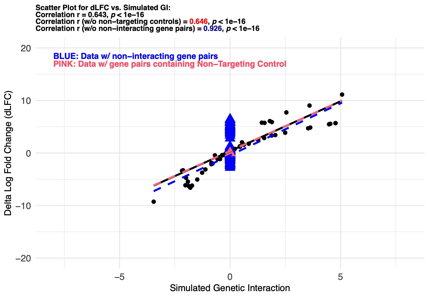
Check relevant details in the pre-built DKOsimR vignettes (PDF) Section 6.
References
[1] Dede, M., McLaughlin, M., Kim, E. et al. Multiplex enCas12a screens detect functional buffering among paralogs otherwise masked in monogenic Cas9 knockout screens. Genome Biol 21, 262 (2020). https://doi.org/10.1186/s13059-020-02173-2.